Contents

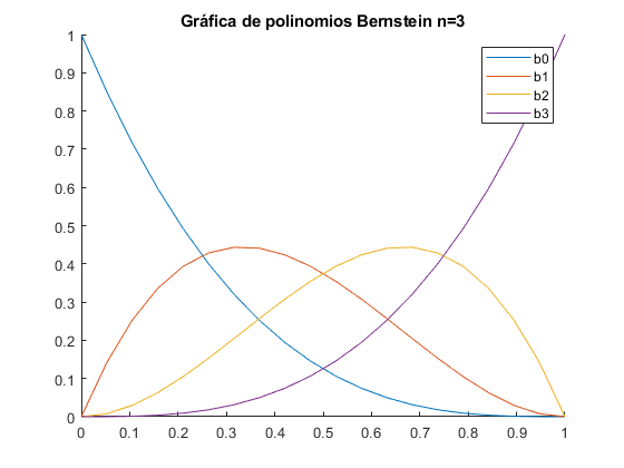
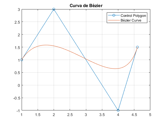
Curva de Bézier

%Las funciones usadas son:

% function factorial_rec=factr(n)
% if n==0
%     factorial_rec=1
% else
%     factorial_rec=n*factr(n-1)
% end

% function c=combina(n,i)
% c=factr(n)/(factr(i)*factr(n-i));
% end

% function b=bernstein(n,i,t)
%     b=combina(n,i)*t.^i.*(1-t).^(n-i);
% end

tb=linspace(0,1,20);
n=3;
figure;
for i=0:3
    b=bernstein(n,i,tb);
    hold on;
    plot(tb,b);
end
legend('b0','b1','b2','b3')
title('Gráfica de polinomios Bernstein n=3')

%...........


t=linspace(0,1,100);
Vx=[1, 2, 4, 4.6];
Vy=[1, 3, -1, 1.5];
V=[Vx;Vy];
figure;
plot(V(1,:),V(2,:),'-o');
n=size(V);
n=n(2);
s=size(t);
x=zeros(n,s(2));
y=zeros(n,s(2));
for i=1:n
    x(i,:)=bernstein(n-1,i-1,t)*V(1,i);
    y(i,:)=bernstein(n-1,i-1,t)*V(2,i);
end
a=sum(x);
b=sum(y);
hold on;
grid on;
plot(a,b);
legend('Control Polygon','Bézier Curve');
title('Curva de Bézier');
hold off
clear all

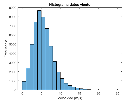
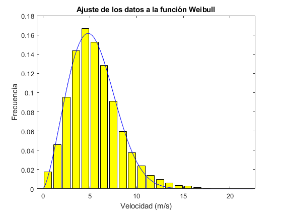
Análisis de la velocidad del viento

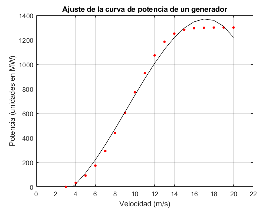
%Histograma datos viento
datos_viento=xlsread('sotaventogaliciaanual.xlsx');
intervalos=0:1:25;
figure;
histogram(datos_viento,intervalos);
title('Histograma datos viento');
xlabel('Velocidad (m/s)');
ylabel('Frecuencia');
hold off;

%Ajuste a la funcion Weibull
velocidad=xlsread('sotaventogaliciaanual.xlsx');
%interpolar si es necesario
if any(isnan(velocidad)) %si hay algún NaN
    x=1:length(velocidad);
    i=find(~isnan(velocidad));
    velocidad=interp1(x(i),velocidad(i),x);
end

x=0.5:1:max(velocidad);
% horas=histogram(velocidad,x);
horas=hist(velocidad,x);
%convierte a frecuencias y ajusta a la función de Weibull
frec=horas/sum(horas);
f=@(a,x) (a(1)/a(2))*((x/a(2)).^(a(1)-1)).*exp(-(x/a(2)).^a(1));
a0=[2 8];  %valor inicial de los parámetros
af=nlinfit(x,frec,f,a0);

%diagrama de frecuencias
figure;
bar(x,frec,'y');
hold on;

%representa la curva de ajuste
x=linspace(0,max(velocidad),100);
y=f(af,x);
plot(x,y,'b')

title('Ajuste de los datos a la función Weibull')
xlabel('Velocidad (m/s)')
ylabel('Frecuencia')
hold off

%APARTADO C
%Interpolar la curva de potencia del generador

Pr=1300; x0=3.0;xr=20;x1=25; %datos de la curva de potencia
potencia=xlsread('sotavento_curva potencia.xlsx','B2:B27');
x=0:1:25;
pot=potencia(x>=x0 & x<=xr);
x=x0:1:xr;
figure;
plot(x,pot,'ro','markersize',3,'markerfacecolor','r')
title('Ajuste de la curva de potencia de un generador');
axis([0 22 0 1400]);
xlabel('Velocidad (m/s)');
ylabel('Potencia (unidades en MW)');
grid on;
hold on;

%ajuste
p=polyfit(x,pot',3); %ajuste a un polinomio de tercer grado
yp=polyval(p,x);
plot(x,yp,'k')
hold off
%cálculo de la potencia media
k=2.3849; c=6.0208; %Parámetro de wwibull calculados antes
f=@(x) (k/c)*((x/c).^(k-1)).*exp(-(x/c).^k); %función de Weibull
h=@(x) f(x).*polyval(p,x);
power=quad(h,x0,xr)+Pr*quad(f,xr,x1);
fprintf('La potencia media (MW) es: %3.1f\n',power)

La potencia media (MW) es: 203.4

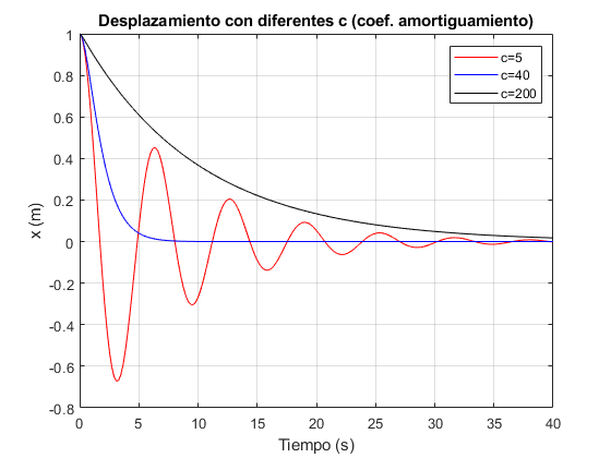
Movimiento muelle

[t1, xx1]=ode45(@muelle, [0,40], [1,0],[ ], 5);
plot(t1,xx1(:,1),'r')

hold on

[t2, xx2]=ode45(@muelle, [0,40], [1,0],[ ], 40);
plot(t2,xx2(:,1),'b')
grid on;
[t3, xx3]=ode45(@muelle, [0,40], [1,0],[ ], 200);
plot(t3,xx3(:,1),'k')
xlabel('Tiempo (s)');
ylabel('x (m)');
title('Desplazamiento con diferentes c (coef. amortiguamiento)');
legend('c=5','c=40','c=200');

% funcion muelle
% function x=muelle(t,x,c)
% x=[x(2); (-c*x(2)-20*x(1))/20];
% end

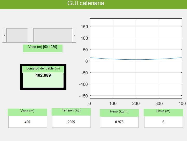
Catenaria

Este programa solo se ejecuta en el .zip

figura_catenaria

Published with MATLAB® R2019b